How To Use VLOOKUP In Microsoft Excel

"VLOOKUP" in Microsoft Excel.

MS Excel formulas: The easiest way to understand Syntax and usage: The most important and magical MS Excel formula is VLOOKUP. It's a great and very useful formula. Without Vlookup knowledge in Excel is like a person without a soul. We use Vlookup very often when we make reports in Excel. Let's start.. 

Formula:  “VLOOKUP"
Explanation:  "VLOOKUP" The most important and most useful formula in Microsoft Excel.

The Use of "VLOOKUP" is to search a value respectively as per input (value in the first column, must match with both sheets or workbooks)

Please follow the given below steps to understand, how to use VLOOKUP.

Step- 1 - Normal Data. Suppose we have some data in Microsoft excel Report - A.  

Report-A

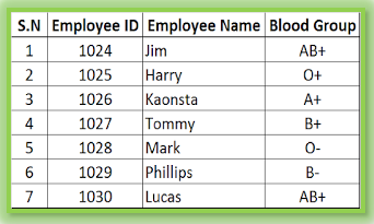
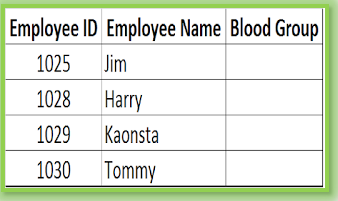
Step: 2 - We have to search for some data from report A to Report B. Suppose we have to search the blood group from report A.

Report-B

Step : 3 - In order to find out the data from Report A to Report B, We can use VLOOKUP" formula. But before using VLOOKUP", we must understand some fact of "VLOOKUP".

Syntax :

=Vlookup (lookup values, Table Array, Col_Index_Num,[range lookup)

Understand the logic of "VLOOKUP".

Lookup value: it is an input. In both sheets, we must have the same value. Employee ID is common and unique for both sheets, with the help of Employee ID we can search the respective data. You can see in the above both sheets the employee no is common.

Table Array: A table array is a selected table, in which we have to pull the data. it will be Report A.

Col_Index_Num: You have to put a number, like 1, 2 , 3 ... etc. You must count the rows starting from the first row you have selected. (Employee ID is called one 1, Employee name is called 2, Blood Group is called 3. In the above example, we are searching Blood Group, so we have to put 3 in Col_Index_Num .

[range lookup] : Range Lookup will be zero or one (0, 1), indicates True and False. Mostly we use 0 (zero)

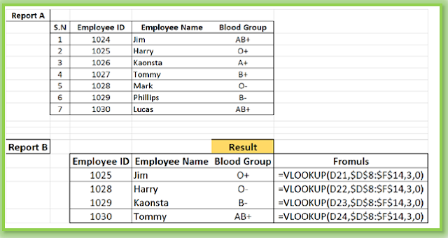
Have a look of the used formula.

=vlookup(D21,$D$8:$F$13,3,0)

Formula Explanation:
 D21 is the input from Report B
$D$8:$F$13 : is the Table Array, from Report A, we have to select from Employee ID to Blood Group until the end of the table.
3: Three is the Col_Index_Num from Report A. We need a blood groups from Report A to Report B and the Blood Group is on the third Row in Report A. So we have to put row no 3.
0: Zero will give you the exact match from the list.

Point To Be Remember:

For a good understanding, prepare the same reports and use the same formula, so can understand the logic of "VLOOKUP".
You must understand the lookup value should be the same in both sheets or reports and your table array should start from the lookup value area.